From BIM databases to Modelica – Automated simulations of heating systems

Keywords: BIM, Modelica, HVAC, simulations

Introduction

There is a large discrepancy between the estimated energy consumptions of buildings and the one measured, often leading to underestimated energy consumption [1, 2]. The issue, known as the performance gap, has many causes. One significant cause is the precision of building energy performance simulations (BEPS) used to estimate energy consumption. BEPS tools rarely consider HVAC systems in detail [3] or simply assume ideal performance of components and controls [4]. This means that commonly occurring phenomena such as oscillation or system imbalance, that create disturbances, are not identified by the BEPS models.

Modeling HVAC systems in detail ensures that all non-ideal performance is considered in the BEPS simulations, which increases simulation precision. In the design phase, this can help to evolve the design process from a steady-state practice, where the design of HVAC systems is based on a worst-case full-capacity situation, to a dynamic design paradigm, where requirements for part-load conditions and dynamic behavior define the design. Additionally, it will be possible to check that the detail of the design is sufficient for actual operation under all conditions. Today, this is ensured through guidelines provided by component manufacturers and empirical knowledge of practitioners. During operation, the detailed models can be used as digital twins for live monitoring of building performance.

Modeling HVAC systems can, however, be a laborious task with many manual processes. Often, the simulation models are built from diagrams of the systems, that the simulation engineer manually interprets and translates to the simulation model format. This error-prone process results in two separate models where changes to one does not affect the other.

Generating the HVAC simulation models from BIM data eases the burden of modeling. Integrating BIM and BEPS ensures that the BIM and simulation models share similar information. Several tools for using BIM as a basis for models in the open-source Modelicalanguage [5] exist [6–8], but all of these have a primary focus on the envelope and thermal zone model. IFC2Modelica[8] includes an example for ventilation systems.

Common for all BIM to BEPS methodologies is their dependence on file-based BIM information. Several critics argue that the use of file-based BIM models limits interoperability and propose a change to web-based collaboration, where information is exchanged through open data formats and stored in centralized databases [9, 10]. This corresponds to BIM level 3 in the Bew-Richards BIM maturity model described in [11], where information exchange is handled through standardized, open data formats for integration with various tools.

Cloud BIM platform

The toolchain, presented in the following sections, is implemented in a cloud platform that stores BIM models in a database to allow cross-platform access to the models. The platform is built with a micro-service structure, which means that several micro-services for design and evaluation of HVAC systems can utilize the data. Amongst these is the Modelica micro-service, which creates models in Modelica language and simulates them with Dymola. As seen in Figure 1, the data flows back and forth between the micro-service and the database so that results are read and analyzed in the platform for analysis and visualization in the graphical user interface (GUI).

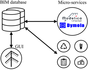
Figure 1. Several micro-services in addition to the Modelica service interface the BIM database platform.

In the database, components and their relations are defined with the Flow Systems Ontology (FSO) [12, 13]. This ontology uses class hierarchies to define the type of component and its relation to other components. E.g., a pipe supplying water to a radiator would have the class Segment and have the property ConnectedWith equal to the radiator's unique tag. Selected classes relevant to this project are listed in Table 1, whereas the full list of classes and connections can be found online in [13].

Table 1. Selected component classes.

Toolchain

The toolchain automatically generates and simulates Modelica models of heating systems from BIM data. In Figure 2the main processes of the toolchain are shown along with the flow of data. On the left side, the tool is connected through an API (see Figure 3), that establishes an integration between the micro-service and the database. As seen in Figure 3 the JSON format is used to parse data between the database and tool. As seen in Figure 2 this is maintained throughout the tool, except for the last two steps, where the simulation environment needs a Modelica file and writes the results to a .mat file. Model data and results are sent back and forth between the toolchain and database an API, as depicted in Figure 3.

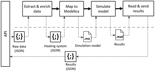
Figure 2. System architecture.

All functions are written with Python, since it is a straight-forward tool which is well suited for translation between data formats and since it is used in the BIM platform. Python does not carry out the simulations itself, but simply interfaces the simulation environment Dymola.

When the toolchain is activated the platform sends a Post request, including BIM data for the desired system(s) to the service's API as seen in Figure 3 where all data exchange between the database, the API and the toolchain is seen.

In the following sections, each step in the tool is described.

Figure 3. Interaction between the database and the toolchain through an API.

System extraction and data enrichment

When activating the tool, BIM data for the heating system is sent from the database, through the API to the tool. As a precaution and for future scenarios with several systems the tool extracts all components in the heating system from the data. To support the following mapping process, minor changes are made to the data by adding certain parameters based on the component classes. E.g., the length of pipe segments is calculated from the component’s start and end coordinates. The enriched/manipulated data is then sent to the mapping process for model generation.

Mapping

In the mapping step, the Modelica models are generated. This is where the original data format and classes are translated to Modelica language and classes. This step is be divided into two separate processes; in the first, the program loops through all components and maps them to a corresponding Modelica class and instantiates it in the model code. In the second, all connections between the components are translated to Modelica connectors. To handle the lack of information on control, this is also where default control connections are established.

In the mapping process, seven FSO classes are mapped to 10 different Modelica classes. Some FSO classes have been mapped to multiple Modelica classes, depending on the value of certain attributes. The full mapping and the translated attributes are seen in Table 2. The parameters are all required in the BIM data; if not, the program will fail.

All Modelica classes, except the bend model, originate from the Buildings library [14] which includes models for most components in HVAC systems in addition to detailed models of thermal zones. To simplify the mapping process, a purpose-built library with models that combine component models from Buildings was created. The combined models simplify the mapping process, since several Modelica models would otherwise have to be instantiated for each database component. Examples are the radiator model, which combines a radiator model and a thermostat, acting as a proportional controller and the MotorValve class, which combines a motorized valve with a PI controller and a setpoint.

Table 2. Mapping between classes in the database and their corresponding Modelica classes.

In the connection process, the connections between components are translated from the database format to Modelica language. In the database, the connection between components are described in connectors, in the ConnectedWith attribute, as seen in Figure 4that shows an example of two connected pipes. All components have at least 2 connectors. Each connector defines the expected direction of flow (in or out) and the connected component's tag, among other properties not relevant to this project.

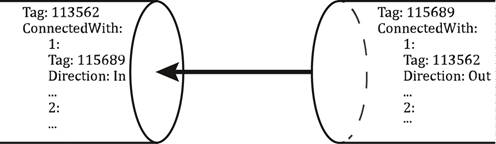
Figure 4. Example of connector definition.

The toolchain loops through all components and for every ingoing connector, a corresponding Modelica connector will be established. Only ingoing connections are considered to avoid duplicate connectors. In Modelica, components are connected through ports. The name of the ports vary depending on the component class, and hence, they are stored in the components during data enrichment.

Since the BIM data does not support definition of control logics, default controls are assumed for the components that need control. E.g., all components mapped to the MotorValve class (see Table 2) control the flow in a heating coil through a PI-controller.

For each component, a component model template is instantiated and added to a text string, containing the model information. After looping through all components, both for class mapping and connection establishment, the text string contains the entire model. The model is saved in a temporary model file for simulation.

Simulation

After mapping, the models are simulated with Dymola through BuildingsPy [15],which interfaces the commercial Modelica simulation environment Dymola. After simulation, the results are parsed to a JSON format and returned to the database.

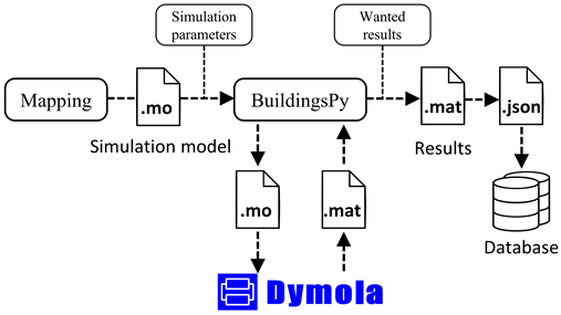
Figure 5. Simulation procedure.

Testing

To ensure that the tool is usable, it was tested on a small heating system model. The test did not focus on assessing the system's performance but merely to check whether the tool works, and the obtained results make sense and are of interest.

Test case description

The test case system, depicted in Figure 6, consists of a heating coil and a radiator, each in separate loops. The main pump supplies flow to both loops, and a secondary pump is connected to the heating coil. To simulate the dynamic behavior, both the heating coil and the radiator are connected to a generic room with the parameters given in Table 3. For simplicity, only heat loss through the walls and window was considered.

The radiator is controlled by a thermostatic radiator valve (TRV), connected to the room temperature. The TRV is not depicted in Figure 6, since it is considered a part of the radiator. To control the heating output of the heating coil, a PI controller adjusts the control valve position to change the heating supply temperature. This is based on the ventilation supply temperature to the room, which has a constant setpoint. For simplicity, both pumps are operated with constant speed, although under normal circumstances, such pumps would either be controlled for constant or proportional pressure. The heat source is not considered, and it is assumed that it supplies water at a fixed temperature of 70°C.

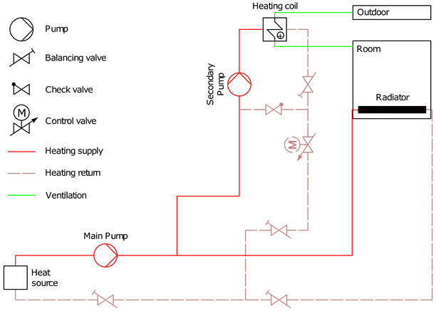
Figure 6. Heating system with one radiator and one heating coil used for testing the tool.

Table 3. Room parameters.

Simulation results

By simulating the system through the toolchain, the overall temperature curves in Figure 7 were achieved. Figure 7shows the temperature of the room and the ventilation supply air, compared to the external temperature. It is seen that the room temperature is stable, but that there is an offset from the setpoint. This offset is caused by the TRV, which in Modelica is modeled as a proportional controller, which will normally introduce an offset. Hence, this behavior is expected. The supply temperature is stable with no offset since it is controlled by a PI-controller.

Additionally, Figure 7 shows the return temperature for both loops and the full system. The return temperatures are stable around 30°C, with a slight tendency to increase with lower external temperatures, as expected.

Discussion and gained experiences

The development process highlighted several points of attention during the mapping process. Most importantly, all needed data for the considered components must be available. If the parameters in Table 2 are not available for all components, the simulations will fail. This puts high demands on the level of information in BIM, but with tools for system dimensioning and component databases, the amount of information is not unrealistic. The possibility to perform detailed simulations of, e.g., return temperatures may even motivate designers to populate BIM models with more information on hydronic components.

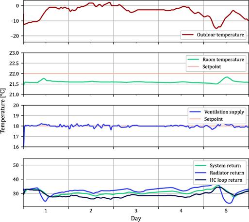
Figure 7. Results for the outdoor (text), room (troom) and ventilation supply (tvent) temperature, including setpoints (SP).

In the presented work, controls were handled by applying a set of assumptions suitable for the specific test case. To work expand the work to larger systems, unambiguous control relations must be established in the database. This can be handled in two ways. Either the existing data format is extended with component parameters for controls, such as process variables, setpoints, etc., or a new data format for controls must be used. Work towards digitizing control information is in growth with several projects under development [9, 16]. Utilizing these existing frameworks to represent control logic in a database seems like a viable solution, but for simpler systems, the simple approach of added attributes may prove sufficient.

The connection between end units and rooms is a vital piece of information to correctly simulate the systems. Creating a link between end units and rooms may be a simple process in the BIM domain, but it requires additional mapping modules to include the rooms in the simulations.

Conclusion and future work

In this paper, it was proved that it is possible to create a tool for the simulation of heating systems based on BIM models. The simulations provided detailed and vital information on the performance of the individual components in the testing case. This showed the value of such simulations that are usually too time-consuming to be made. While the presented results may be trivial for a system as small as the test case, the same analysis for larger system will uncover results that are difficult for normal practitioners to quantify.

Several important attention points for a larger implementation were identified, the biggest being the lack of representation of controls in BIM models. These points resulted in several assumptions built into the tool, especially regarding control strategies. These assumptions mean that the tool is less flexible to different system configurations. By extending the data format to include the needed information on controls, the tool can easily be modified to simulate larger systems with both heating, ventilation, and cooling systems. When this work is done, the full models can be used in fault detection, detailed analysis of the dynamic effects of coupling the systems, etc.

Acknowledgement

This work was funded by the national IFD grant J.nr. 8090-00046B for the project “HEAT 4.0 - Digitally supported Smart District Heating”, Elforsk grant 352-042, IFD grant J.nr. 9065-00266A for the project “Virtual Commissioning in Building Services” and “Databaseret energistyring i offentlige bygninger”, EU Interreg-ÖKS 2020-2022.

References

Please find the full list of references in the original article at: https://proceedings.open.tudelft.nl/clima2022/article/view/365